Gemma4-12B was released by Google a few weeks ago and it piqued my interest as an interp researcher since it diverges from the mainstream paradigm: it is an encoder-free vision-language model that processes image patches and audio segments directly as tokens, without a separate vision or audio encoder. This raises an interpretability question: what do those non-text tokens represent at each layer of the transformer, do they resemble interpretable text representations?
We apply two complementary probes to every visual/audio token at 12 selected layers (1, 4, 8, 12, 16, 24, 28, 32, 36, 40, 44, 47). LatentLens (Krojer et al., 2026; normalized) retrieves the nearest-neighbor tokens from a large caption corpus in the model's own representation space. I had developed this method recently (presenting at ICML in Seoul) and was curious how well it would work here. Interestingly, compared to our original LatentLens, I had to add a normalization step to account for outlier dimensions that otherwise dominate cosine similarity.1 I also apply the more established LogitLens (nostalgebraist, 2020), which projects the raw hidden state through the unembedding matrix to return ranked vocabulary predictions. While LatentLens retrieves corpus tokens by similarity search, LogitLens reads off vocabulary logits directly; comparing both across layers reveals how the model processes non-text modalities.
Explore the demos or read through some findings below.
We manually inspect a handful of PixMo-Cap examples, examining nearest-neighbor predictions for individual patches at 12 selected layers (1, 4, 8, 12, 16, 24, 28, 32, 36, 40, 44, 47).
Layer-by-layer summary of what I found
Layer range
LatentLens (norm.)
LogitLens
Key observation
1–4
nothing
not working
High raw cosine similarity at L4 may reflect a rogue-dimension artifact
8
OCR only
not working
First interpretable signal, exclusively on image text
12
OCR + first semantics
not working
Semantic (non-OCR) content begins appearing
16
~50% patches interpretable
not working
Raw cosine similarities spike to >0.99 for LatentLens (unnorm.) — all corpus tokens look identically similar, so nearest neighbors are meaningless. LatentLens (norm.) is unaffected and peaks here.
24–28
mostly silent
not working
LatentLens loses most signal; only a few OCR patches remain
32
OCR only
not working
OCR retrieval recovers in LatentLens; non-OCR still silent
36
partial, lower diversity
starts working
Partial recovery in LatentLens, but less diverse — same few neighbors recur across patches of the same image
40–44
OCR competitive
leads on semantics; next-token on OCR
LogitLens overtakes LatentLens on general content; on OCR patches LogitLens predicts the next word in image text, not the current one
47
silent
slightly weaker than L44
Both methods degrade; last layer optimized for next-token prediction, not patch decoding
Selected examples
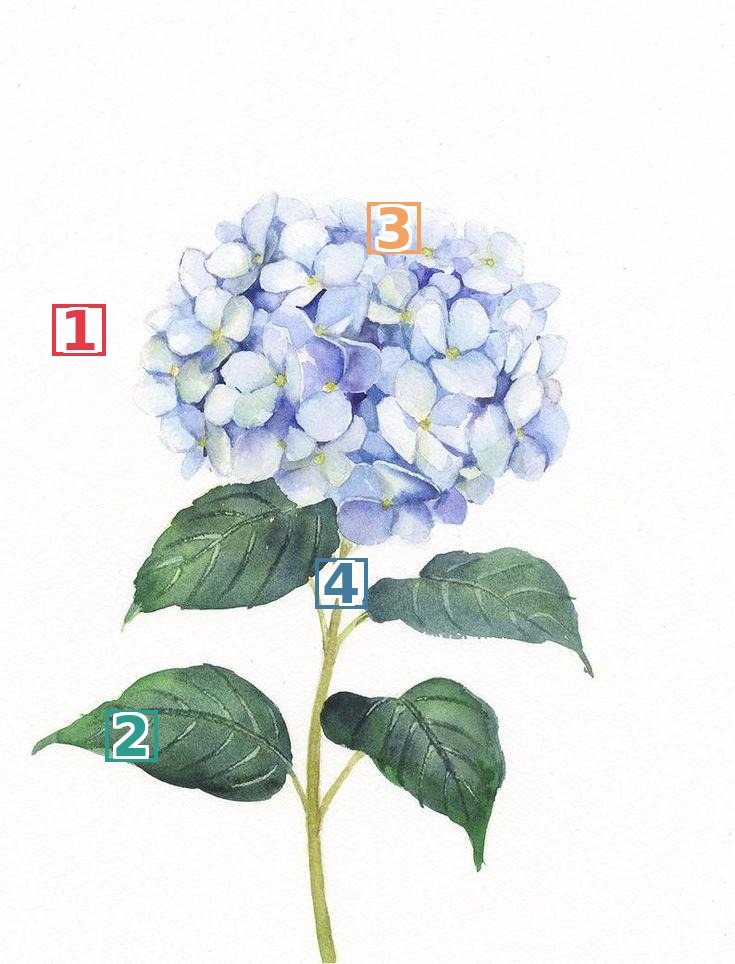
Image 6 in demo (watercolor hydrangea), Layer 16 — semantic predictions across flower, leaf, color, and stem patches
#
Region
LatentLens top predictions (normalized)
1
flower cluster
flowers 0.362flowers 0.287flor 0.286
2
lower leaf
leaves 0.236leaf 0.177foliage 0.167
3
blue petals
blue 0.232Blue 0.229blue 0.224
4
stem
stems 0.150branching 0.134branches 0.118
Patches 1–2 show semantic plant-part recognition; patch 3 shows color perception (“blue”) for the blue-tinted petals; patch 4 identifies the stem structure. No text in the image — all predictions are purely visual.
Any image with visible text, Layers 40–44 (most prominent at 44) — LogitLens predicts the next OCR word, not the current one
On image text, the patch over a word at layers 40–44 has LogitLens returning the following word rather than the current one — e.g. the patch over “final” in “my final exam” returns “exam”. The effect is most prevalent at layer 44. Explore any image with text in the demo to verify.
LatentLens (normalized) and LogitLens are complementary: LatentLens provides the main interpretable signal at layers 8–16, while LogitLens takes over at layers 40–44. Layers 24–28 are largely non-interpretable with LatentLens (norm.) — only a few OCR patches remain; LogitLens does not work here. OCR retrieval in LatentLens partially recovers at L32. At layer 16, raw cosine similarities spike to >0.99 for the unnormalized case — every corpus token looks nearly identical to every query token, so nearest-neighbor retrieval is uninformative. Z-score normalization corrects this.
Audio Tokens
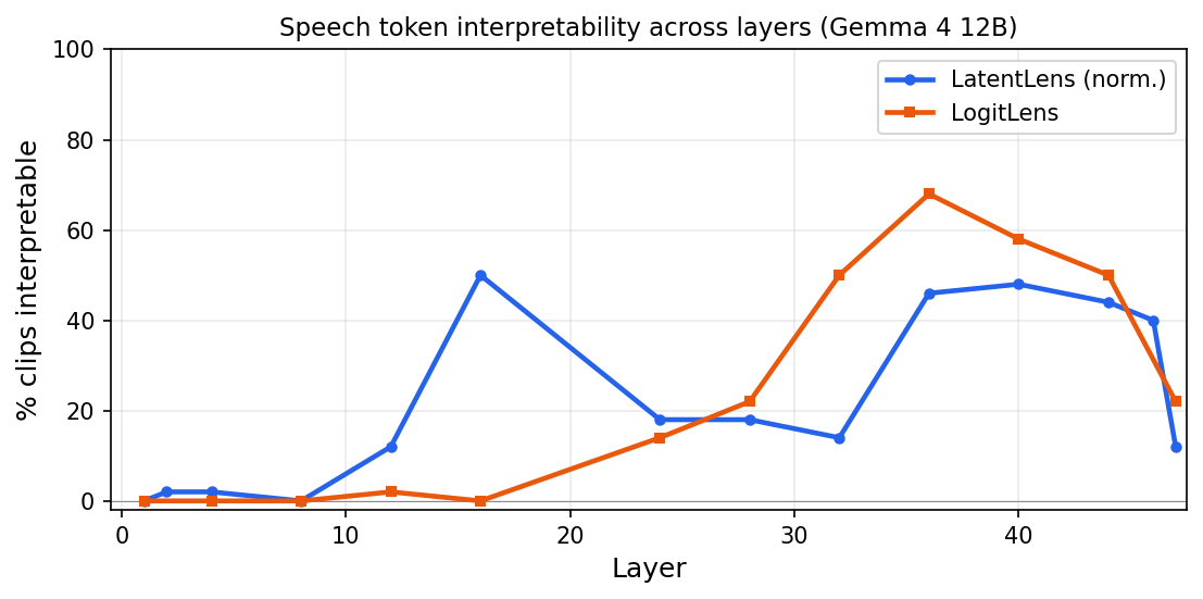
We probe 50 speech clips from LibriSpeech test-clean. Each 40ms audio token is evaluated independently at 12 selected layers. We measure the fraction of clips where any top-5 prediction matches a transcript word.
Percentage of LibriSpeech clips (50 total) where LatentLens (norm.) or LogitLens returns at least one transcript word in the top-5 predictions, measured at two sampled tokens per clip.
LatentLens (normalized) peaks at 50% of clips at layer 16 — the same layer where LogitLens produces no correct predictions at all (0%). LogitLens recovers and overtakes LatentLens from layer 32 onward, peaking at 68% at layer 36.
Environmental sounds (ESC-50). We separately probed 50 environmental sound clips from ESC-50 (one per category: crow, rain, chainsaw, …). This is a much more open-ended scenario than language-centric speech that comes with a transcript. We used an LLM judge to evaluate all 700 clip–layer pairs for any semantic connection to the sound category, yielding only a single hit (!) out of 700: “aerodynamics” for the airplane category at layer 40. All other predictions are unrelated vocabulary (“expressive”, “poetry”, “karate”, “surroundings”) with no connection to the playing sound. Neither LatentLens nor LogitLens revealed interpretable non-speech audio representations at any of the 14 probed layers.
Temporal structure
When inspecting the demo and listening to spoken words, I was surprised that LatentLens predictions for a token often matched a word spoken earlier in the clip, e.g. a token at t=3s would retrieve “concord” even though “concord” was spoken at t=0.5s. The model appears to stay anchored to earlier content words as context accumulates. Yet the order of retrieved words across tokens still matched the transcript order.
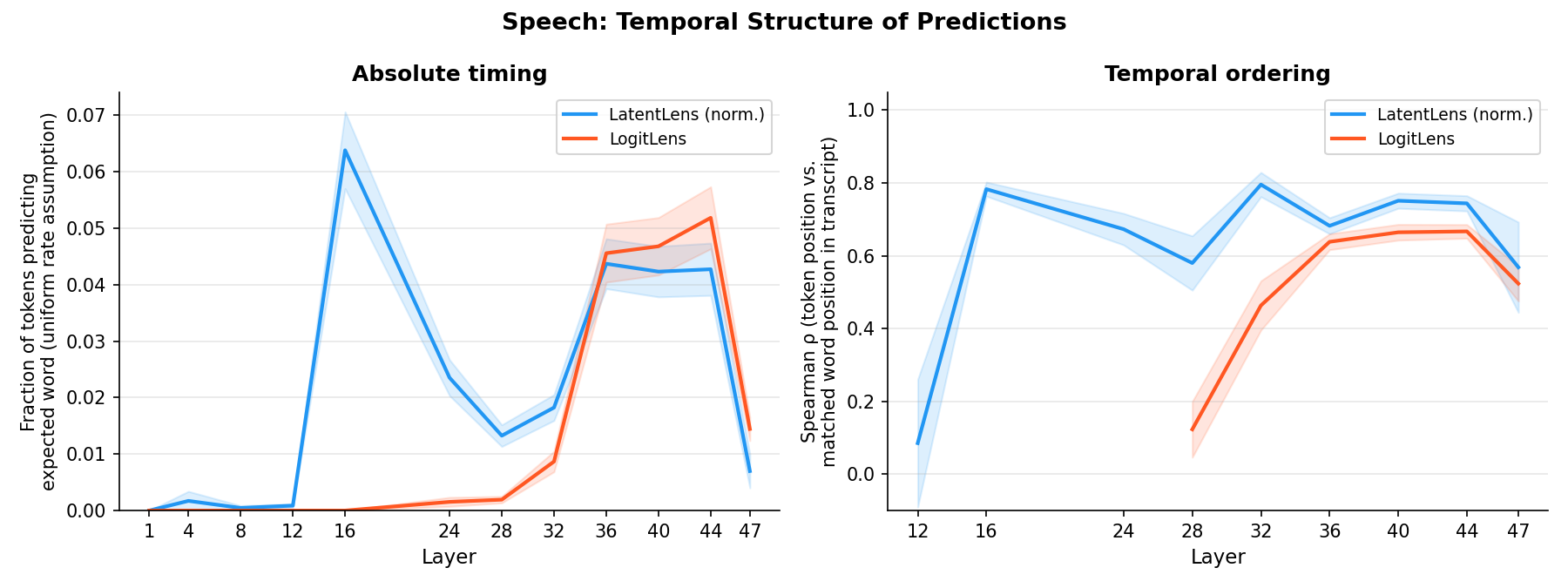
Left: fraction of tokens predicting the specific word expected at that exact timestamp (uniform speech rate assumption). Right: Spearman rank correlation between token position in the clip and matched word position in the transcript, restricted to clips where ≥3 unique words were matched. LogitLens only appears from L28 onward — at earlier layers it produces too few matches to compute the correlation.
Absolute timing (left) is low: at the peak layer (L16), only 6.4% of tokens predict the word expected at that exact timestamp. Temporal ordering (right) is much higher: when predictions do match transcript words, they tend to appear in the correct sequence (Spearman ρ ≈ 0.78 at L16, 0.67–0.75 at L36–44).
In other words: at layer 16, the model has encoded much of the utterance's vocabulary in the correct sequence, but without precise temporal localization. The ordering finding is robust (n=47/50 clips) but not perfect — ρ of 0.78 means substantial ordering with real scatter.
Clip 2 in demo (speech_00000, 3.5s) — transcript: “CONCORD RETURNED TO ITS PLACE AMIDST THE TENTS”
Layer 16, LatentLens (normalized) top predictions, selected tokens:
Token
Time
Top predictions
48
1.92s
concord 0.178ant 0.174
60
2.40s
returned 0.361return 0.318
73
2.92s
place 0.270places 0.241
83
3.32s
amidst 0.265mid 0.184
All four words appear in transcript order, in the second half of the 3.5s clip. The model encodes the full utterance vocabulary before precise timing is established.
Three findings appear consistently across both modalities and both probe methods:
Layer 16 is where rogue dimensions dominate. Raw cosine similarities spike to >0.99, making nearest-neighbor retrieval in LatentLens (unnorm.) uninformative — every corpus token looks equally similar. In audio, LogitLens also predicts no transcript words at this layer (0% match rate). Z-score normalization sidesteps this and LatentLens (norm.) peaks here.
LatentLens and LogitLens are complementary. LatentLens (norm.) provides the main signal in layers 8–16 (50% speech hit rate at L16); layers 24–32 are largely silent, with OCR partially recovering at L32; LogitLens does not work until ~L32 and peaks at L36 (68% speech hit rate). Neither LatentLens nor LogitLens revealed interpretable non-speech audio representations at any of the 14 probed layers.
Speech: Representations encode ordering but not precise timing. For speech at L16, predictions match transcript words in the correct temporal order (Spearman ρ ≈ 0.78 across 47/50 clips) while exact-timestamp alignment is low (6.4%). A somewhat related, more expected, phenomenon appears in vision: at layers 40–44 (most pronounced at L44), LogitLens on OCR patches predicts the next word in image text rather than the current one.
@misc{krojer2026latentlens,
author = {Krojer, Benno},
title = {{Inspecting Visual and Audio Token Representations in Gemma4-12B}},
year = {2026},
month = {June},
url = {https://bennokrojer.com/gemma4-interp/},
note = {Blog post}
}
At several layers — most acutely at L16 — a small subset of hidden-state dimensions have anomalously large variance across tokens (sometimes called rogue dimensions; Timkey & van Schijndel, 2021). Note that a dimension with a large but constant value would not harm cosine similarity — it would cancel between numerator and denominator. The problem is the cross-token variation: some tokens score very high in a rogue dimension while others score low, so cosine similarity becomes dominated by whether two tokens happen to co-activate there, collapsing pairwise similarities to >0.99 for virtually every pair and making nearest-neighbor retrieval degenerate. Z-score standardizing each dimension across all tokens before computing similarities (dividing by per-dimension standard deviation) brings all dimensions to unit variance and resolves this. After normalization, LatentLens actually peaks at L16 rather than failing there. ↑